Partial Pixel Specification VAEs

Autoencoding Conditional Neural Processes for Representation Learning

Conditional neural processes (CNPs) are a flexible and efficient family of models that learn to learn a stochastic process from data. They have seen particular application in contextual image completion - observing pixel values at some locations to predict a distribution over values at other unobserved locations. However, the choice of pixels (context set) in learning CNPs is typically either random or derived from a simple statistical measure (e.g. pixel variance). Here, we turn the problem on its head and ask which context set would a CNP like to observe. We show that Learning to invert conditional neural processes (CNPs) can lead to selection of meaningful subsets of data.

ICML 2024

Partial Pixel Space (PPS)

From the frame of representation learning, the context set (observed pixels) can be viewed as latent representations of the image - one that happens to exist in the data space. We call such latent representation Partial Pixel Space (PPS).

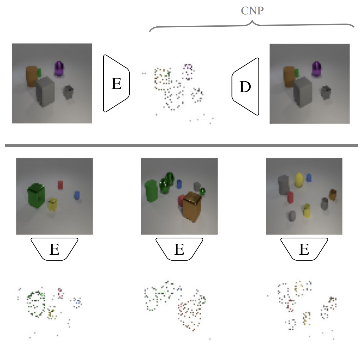
Here, we develop the Partial Pixel Space Variational Autoencoder (PPS-VAE), an amortised variational framework that casts CNP’s context set (PPS) as latent variables learnt simultaneously with the CNP (see Figure 1).

PPS-VAE

To answer our question of what kinds of context set the CNP would like to observe, we first cast the CNP as a fully generative model (Figure 2, left - yellow area):

\begin{equation} p_\theta(\mathbf{x}, \mathbf{y} \mid M) = p_\theta(\mathbf{x_M}) p_\theta(\mathbf{y_M} \mid \mathbf{x_M}) p_\theta(\mathbf{y_T} \mid \mathbf{x_T}, \mathbf{x_M}, \mathbf{y_M})\nonumber, \end{equation}

where $M$ is taken to be a given fixed value, $p_\theta(\mathbf{x}_M)$ defines a distribution over arrangements of $M$ pixel locations in an image, $p_\theta(\mathbf{y}_M\mid\mathbf{x}_M)$ a distribution over values at the given locations and $p_\theta(\mathbf{y_T} \mid \mathbf{x_T}, \mathbf{x_M}, \mathbf{y_M})$ a distribution over values at the unseen locations $\mathbf{x_T}$.

The model can be viewed as generating data in two stages (autoregressive): first generating the values corresponding to the context points $(\mathbf{y}_M,\mathbf{x}_M)$, and subsequently, conditioning on these locations and values to impute the values elsewhere on the image.

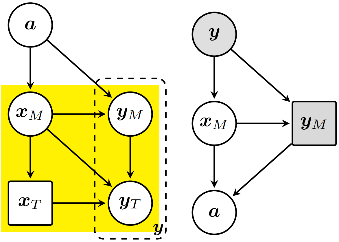
Figure 2: CNP generative model (left yellow); PPS-VAE generative (left) and inference (right) models

To get to the full PPS-VAE generative model, we additionally introduce an abstractive latent variable $\mathbf{a}$:

\begin{equation} p_\theta(\mathbf{a}, \mathbf{x}, \mathbf{y}| M)= p_\theta(\mathbf{a})\; p_\theta(\mathbf{x_M} | \mathbf{a})\; p_\theta(\mathbf{y_M} | \mathbf{x_M}, \mathbf{a})\; p_\theta(\mathbf{y_T} | \mathbf{x_T}, \mathbf{x_M}, \mathbf{y_M})\nonumber \end{equation}

The latent variable $\mathbf{a}$ acts as an abstraction of the context set/PPS, providing smooth control over different arrangements and values, while also allowing the model to flexibly learn the mapping between arrangement of pixel locations and corresponding pixel vales.

The standard CNP formulation estimates the marginal $p_\theta(\mathbf{y}|M)$ by sampling uniformly at random from $p(\mathbf{x}_M)$. One can instead construct a more informative importance-sampled estimator by employing a variational posterior $q_\phi(\mathbf{x}_M \mid \mathbf{y}, M)$: \begin{equation} q_\phi(\mathbf{a}, \mathbf{x_M} |\mathbf{y}, M) = q_\phi(\mathbf{x_M} | \mathbf{y})\; q_\phi(\mathbf{a} | \mathbf{x_M}, \mathbf{y_M})\nonumber \end{equation}

Crucially, given a means to generate locations $\mathbf{x}_M$, one can simply lookup the image $\mathbf{y}$ at those locations to derive $\mathbf{y}_M$—an observation itself—as shown in Figure 2 (right). From a representation-learning perspective, the context set can be seen as a partial pixel specification of the image.

Putting the generative and inference models together, we construct the variational evidence lower bound (ELBO) as:

\begin{equation} \log\ p_\theta(\mathbf{y}|M) \nonumber \geq E_{q_\phi(\mathbf{a}, \mathbf{x_M} |\mathbf{y}, M)} \left[ \log \frac{p_\theta(\mathbf{a}, \mathbf{x}, \mathbf{y}| M)}{q_\phi(\mathbf{a}, \mathbf{x}_M |\mathbf{y}, M)} \right] \label{eq:ppsvae-elbo} \end{equation}

Utility of Method

Utility 1 - Visual inspection of PPS in image space without post-hoc approaches.

Since there is 1-to-1 correspondence between pixels in the context set an the original image it allows us to perform a qualitative observation of the chosen pixels and put forward hypothesis regarding how PPS-VAE abstracts information for different settings of $M$. Results are shown in Figure 3.

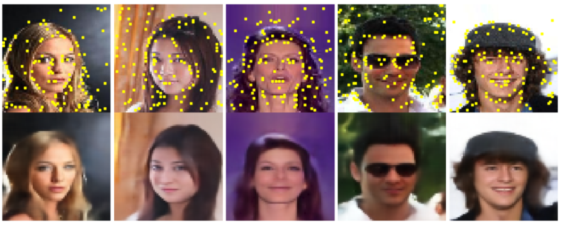
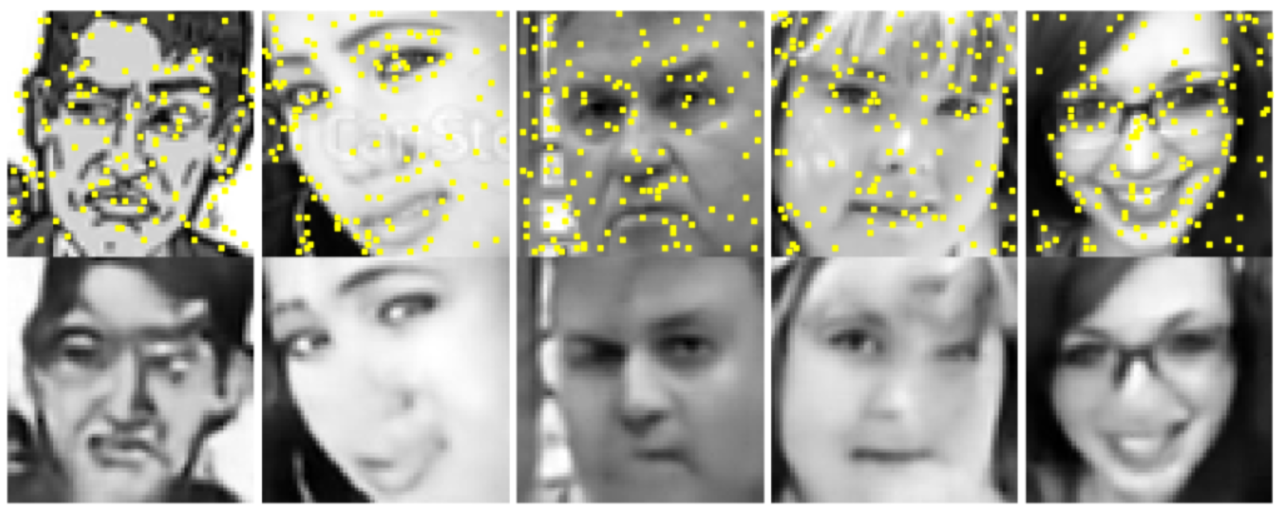
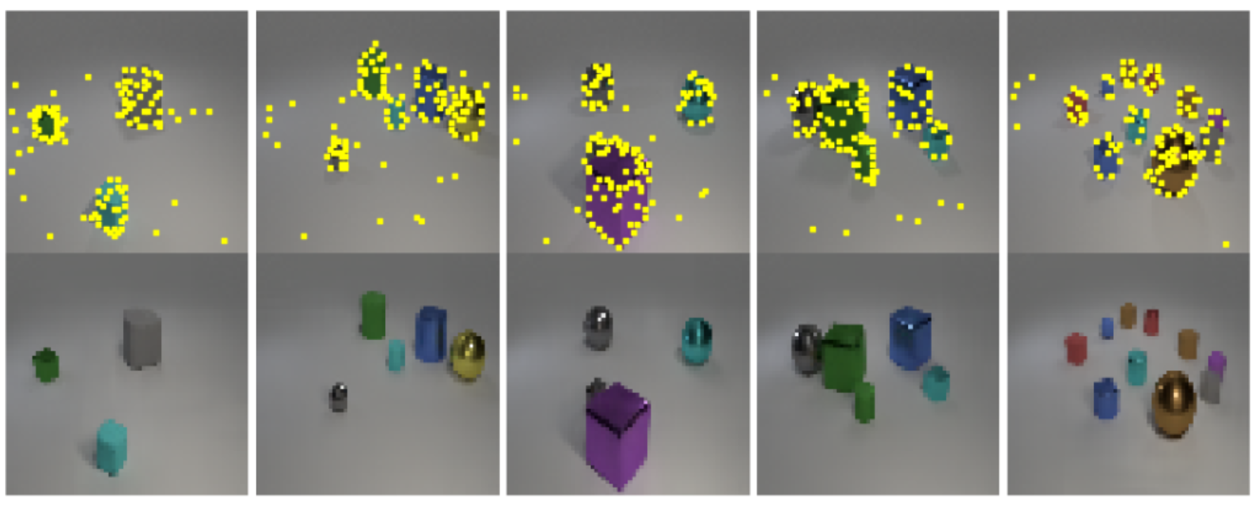
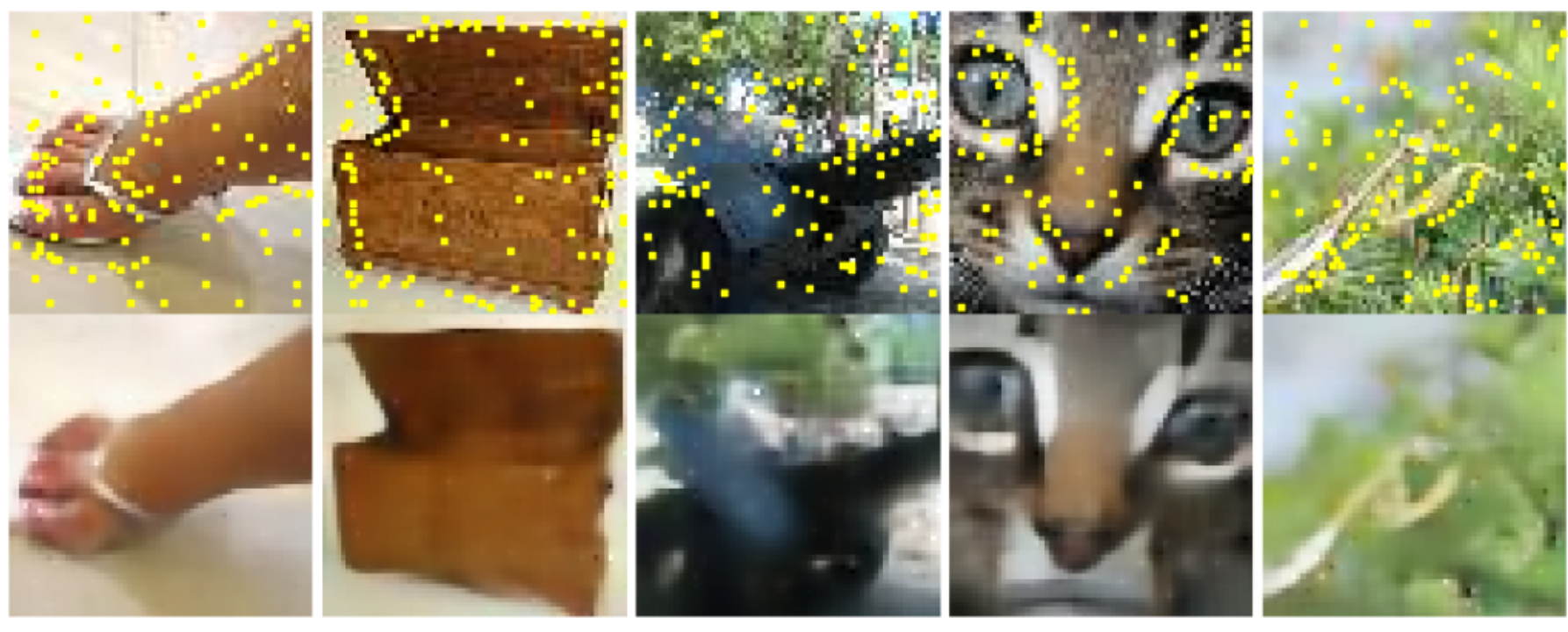
Figure 3: PPS-VAE induced context points for different datasets

The patterns that context sets form can be summarised with the following observations: (1) boundary points between objects and the background generally describe shape, (2) points on the object can capture `interior’ colour, and part locations and (3) background points capture complexity outside the objects (e.g. uniform colour etc.).

Utility 2 - Change representational capacity of PPS at inference time.

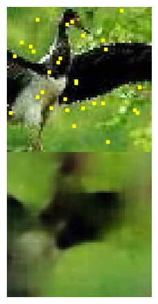
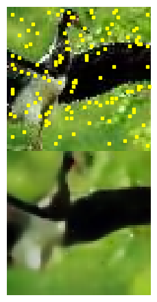
A differentiating property of our model is the ability to increase the capacity of the latent representation (PPS) at inference time. We can encode more information in the context set by simply increasing $M$, without retraining the model. We propose two ways of doing this: (1) simply increase $M$ at inference time (see Figure 4) and (2) augment $\mathbf{y}_M$ at inference time by adding to each pixel in $\mathbf{y}_M$ 8 neighbouring pixels - creating 3x3 tiles after pre-training (see Figure 5).

Figure 4: Inference-time adaption of context-set size ($M$)

Utility 3 - PPS can provide better features for a classifier than an original image.

Having observed that the context sets/PPS do indeed appear to capture meaningful features, we conduct further analyses to quantify how meaningful they can be. We do this through the lens of classification, by probing the context set/PPS $\mathbf{y}_M$ to see how well it captures class-relevant information. Here we report the results for the two out of the four datasets that we use. Check the paper for the remaining two

Probing reveals that (1) the context set preserves class label information which is on par or better than baselines (2) augmented or increased capacity PPS provides better features for the classifier than the original image on CLEVR dataset.

Models	CLEVR	t-ImageNet
PPS-RAND	36.17 $\pm$ 3.39	21.86 $\pm$ 0.31
VQ-VAE	75.91 $\pm$ 0.47	29.02 $\pm$ 0.08
FSQ-VAE	73.27 $\pm$ 0.36	31.03 $\pm$ 0.40
PPS-VAE (points)	90.21 $\pm$ 0.28	29.56 $\pm$ 0.27
PPS-VAE (points) 128->256	`93.38` $\pm$ 0.64	33.93 $\pm$ 0.16
Image	91.90 $\pm$ 0.30	`43.68` $\pm$ 0.03